There are deep learning models that are pre-trained on millions of image data. These models reduce the effort to train the custom deep learning model from scratch, you need to fine-tune them and they are ready to be trained on your dataset.

Keras provides a high-level API for using pre-trained models. You can easily load these models with their pre-trained weights and adapt them to your specific tasks by adding custom classification layers on top of the pre-trained layers. This allows you to perform transfer learning efficiently.

In this article, you’ll see which of the four commonly used pre-trained models (VGG, Inception, Xception, and ResNet) is more accurate with their default settings. You’ll train these models on the image dataset and at the end you will able to conclude which model performed the best.

Model Name	Top-1 Accuracy	Top-5 Accuracy	Parameters
VGG16	71.3%	90.1%	138.4M
Xception	79.0%	94.5%	22.9M
ResNet50	74.9%	92.1%	25.6M
InceptionV3	77.9%	93.7%	23.9M

You can see that the Xception has the highest top-1 and top-5 accuracy among these models and it is trained on 22.9 million data points.

Evaluating the Accuracy of Pre-trained Models

In this section, you’ll train the aforementioned models on the cats and dogs image dataset and evaluate the accuracy.

Importing Required Libs and Modules

All the modules and classes that will be required throughout this article are imported.

• Sequential will be used to lay the architecture of the model.
• Dense layer will be used to add the fully connected layer, Flatten will be used for flattening the layer to 1D, GlobalAveragePooling2D will be used to reduce the dimensions of neural networks, and Dropout will be used to regulate the neurons by randomly shutting the neurons to avoid overfitting.
• Pre-trained models (Xception, InceptionV3, VGG16, and ResNet50) are imported from the tensorflow.keras.applications module.
• ImageDataGenerator will be used for preprocessing the images.
• accuracy_score will be used to determine the accuracy of the models on the test dataset.

Train, Test & Valid Directory Paths

The dataset is divided into three directories: train, valid, and test, with two subdirectories within each: cat and dog.

The full path to each of these directories is specified: train_path holds training data, valid_path holds validation data, and test_path holds testing data.

Preprocessing Image Data

The ImageDataGenerator is used to preprocess images for training, validation, and testing datasets.

The images will be rescaled to have pixels between 0 and 1. More specifically, resacle=1.0/255.0 means that each input image’s pixel value will be divided by 255 to scale down the pixel values.

Setting Up Data Generators

This step involves creating data generators for training, validation, and testing data.

The first line of code uses the flow_from_directory() method to generate training data with the following parameters:

• directory=train_path: Training directory path from where the images will be loaded.
• traget_size=(224,224): This resizes the image dimensions into 224×224 pixels.
• classes=['cat', 'dog']: Defines the classes for classification.
• batch_size=10: The generator will produce batches of 10 images at a time.

Similarly, this process will be repeated for validation and testing data. However, because the shuffle parameter is set to False, testing data will not be shuffled.

As you can see, 1000 images belong to 2 classes i.e., “cat” and “dog” (500 images for each class) found in the train directory. The valid and test directories found 200 and 100 images respectively.

Initializing Models

The pre-trained models are initialized (VGG16(), Xception(), InceptionV3(), and ResNet50()) with the parameters are as follows:

• include_top=False: This means that the fully connected layers will not be included at the top of the neural networks.
• input_shape=(224, 224, 3): The pre-trained models are initialized with the input shape of the images set to 224x224 with the RGB (3) color channel.

Freezing the Layers

The above code loops through the list of pre-trained models stored in the names variable, and then the inner loop iterates through the layers of each pre-trained model, freezing them by setting the trainable layer to False (layer.trainable = False).

This step is included because the layers have already been trained and it is pointless to train them further during fine-tuning. That is the entire purpose of employing the transfer learning technique.

Fine-tuning the Pre-trained Models for Transfer Learning

The number of classes present in the training dataset is determined using the len(train_gen.class_indices) and stored inside the output_classes variable.

A new Sequential model (custom_vgg_model) is constructed with the pre-trained VGG16 model and custom layers are added to it. The layers are flattened to a 1D vector using the Flatten() layer followed by a fully connected (Dense) layer with 256 neurons and an activation function “ReLu” is added. Then a Dropout layer with a rate of 0.5 (50%) is added regulating the neurons in the neural network and finally, an output layer (Dense) is added with output_classes and activation function “Softmax”.

A custom model custom_xc_model is constructed with a pre-trained Xception model (model_xception). A GlobalAveragePooling2D layer is added to reduce the dimensionality of the model and an output layer (Dense) is added with output_classes and activation function “Softmax”.

Similarly, custom_inc_model and custom_resnet_model are constructed with pre-trained InceptionV3 (model_inception) and ResNet50 (model_resnet) models respectively.

Compiling Models with Optimizer, Metrics and Loss

A list called models is defined that contains a collection of fine-tuned models.

A loop is created that iterates through the models in the list, and each model is compiled with an optimizer named "Adam", the loss is computed using 'categorical_crossentropy', and the 'accuracy' is used as metrics to measure the accuracy.

Training the Models

A list (model_names) is created in which each item is a pair that consists of a fine-tuned model (e.g. custom_vgg_model) and model name (e.g. “VGG16”).

A loop is created that iterates through the fine-tuned model and associated model name from the list model_names. The model.fit() method is called to train each model with the following arguments:

• train_gen: Training data generator that will provide batches of training data on which the model is going to be trained.
• validation_data=valid_gen: Validation data generator that will be used to check the performance of the model on the validation set without actually training on it.
• epochs=10: The model will train for 10 epochs which means the model will train the entire training set 10 times.
• verbose=0: This will not show any progression on the screen.

Then the model predicts on the test_gen data using the model.predict() method and store the results inside the test_pred.

Following that, the actual test labels are collected using the test_gen.classes and stored inside the test_labels variable. This will be used to compare against the predicted labels.

In the final step, the accuracy of the models is evaluated using the accuracy_score. The accuracy is determined by comparing the true test labels (test_labels) with predicted test labels (np.argmax(test_pred, axis=1)).

Here, np.argmax(test_pred, axis=1) is used to pick out the max element from the array (test_pred). Using this, you get the array of class labels 0 and 1.

Result

When you run each model for 10 epochs on the training dataset, the following accuracy on the test data is obtained:

• VGG16: 91%
• Xception: 100%
• InceptionV3: 99%
• ResNet50: 62%

As can be seen, the Xception model performed exceptionally well and achieved 100% test accuracy, whereas the ResNet50 model struggled to learn and achieved 62% test accuracy.

You can try out different pre-trained models and datasets. During fine-tuning, you can also experiment with increasing the number of epochs or adding more fully connected models.

Please keep in mind that your results may vary depending on the various factors.

Visualizing Train and Valid Accuracy

You can determine the learning curve for each model by visualizing the training and validation accuracy for each epoch.

Adjust the above code as shown below:

The above code will produce the following image showing the plots for each model that contains two lines: training accuracy and validation accuracy:

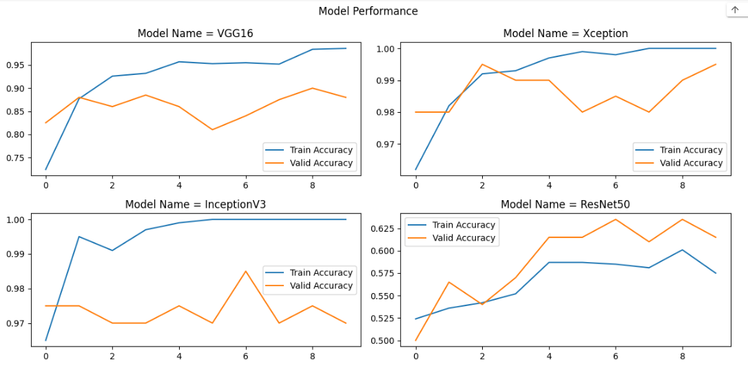
Using the plot above, you can examine the training and validation accuracy of each model. As can be seen, the InceptionV3 model achieved 100% test accuracy around the 5th epoch, while the Xception model achieved 100% test accuracy around the 7th epoch.

Conclusion

In this tutorial, you’ve seen commonly used (VGG, Xception, Inception, and ResNet) pre-trained models are fine-tuned and then trained on the image dataset to see their performance on the test data.

---

🏆Other articles you might be interested in if you liked this one

✅How do learning rates impact the performance of the ML and DL models?

✅How to build a custom deep learning model using transfer learning?

✅How to build a Flask image recognition app using a deep learning model?

✅What is StandardScaler() in ML and why it is used?

✅How to perform data augmentation for deep learning using Keras?

✅Upload and display images on the frontend using Flask in Python.

---

That’s all for now

Keep Coding✌✌