Introduction

Transfer learning is used in machine learning and is a method in which already-trained or pre-trained neural networks are present and these pre-trained neural networks are trained using millions of data points.

This technique is currently most famous for training deep neural networks because its performance is great when training deep neural networks with less data. Actually, it’s instrumental in the data science field because most of the real-world data typically do not have millions of data points for training a robust deep learning model.

Numerous models are already trained with millions of data points and can be used for training complex deep-learning neural networks with maximum accuracy.

Ahead in this tutorial, you’ll learn to train deep neural networks using the transfer learning technique.

Keras applications for transfer learning

Before building or training a deep neural network, you must know what are options available for transfer learning and which one you must use to train a complex deep neural network for your project.

Keras applications are deep learning models that have pre-trained weights that are used for predictions, feature extraction, and fine-tuning. There are numerous models present in the Keras library and some of the popular models are

Xception
VGG16 and VGG19
ResNet Series
MobileNet

Discover More on Keras Application.

In this article, you’ll see the use of the MobileNet model for transfer learning.

Training a deep learning model

In this section, you’ll learn to build a custom deep-learning model for image recognition in a few steps without writing any series of layers of convolution neural networks (CNN), you just need to fine-tune the pre-trained model and your model will be ready to train on the training data.

In this article, the deep learning model will recognize the images of the hand sign language digits. Let’s start building a custom deep-learning model.

Grab the dataset

To start the process of building a deep learning model, you will need the data first and you can easily choose the right dataset from millions of datasets by visiting a website called Kaggle. Though there are other websites also that provide datasets for building deep learning or machine learning model.

But the dataset that will be used in this article is taken from the Kaggle named American Sign Language Digit Dataset.

Data preprocessing

After downloading and saving the dataset into the local storage, now it’s time to perform some preprocessing on the dataset like preparing the data, splitting the data into train, valid, and test directories, defining their path, and creating batches for training purposes.

Preparing the data

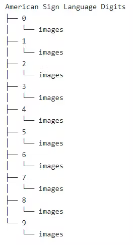
When you download the dataset, it contains directories from 0 to 9 in which there are three sub-folders input images, output images, and a CSV folder for each directory.

Go ahead and remove the output images and CSV folder from each directory and move the content of the input images to the main directory and then remove the input image folder.

Each main directory of the dataset now have 500 images, it’s your choice to keep all the image but for demonstration purposes, only 200 images will be used in each directory in this article.

The structure of the dataset will look as shown in the image below.

Splitting dataset

Now let’s start by splitting the dataset into the train, valid, and test directories.

The train directory will contain training data which will be the input data that we feed into the model for learning the pattern and irregularities.

The valid directory will contain the validation data that will be infused into the model and will be the first unseen data that the model has seen and it will help in getting maximum accuracy.

The test directory will contain the testing data that will be used for testing the model.

Import the libraries that will be used further in the code.

# Importing required libraries

import os

import shutil

import random

Here’s the code that will make the required directories and move the data into the specific directories.

# Creating dirs train, valid and test and organize data into them

os.chdir('D:\SACHIN\Jupyter\Hand Sign Language\Hand_Sign_Language_DL_Project\American-Sign-Language-Digits-Dataset')

# If dir doesn't exist then make specified dirs

if os.path.isdir('train/0/') is False:

os.mkdir('train')

os.mkdir('valid')

os.mkdir('test')

for i in range(0, 10):

# Moving 0-9 dirs into train dir

shutil.move(f'{i}', 'train')

os.mkdir(f'valid/{i}')

os.mkdir(f'test/{i}')

# Take 90 sample imgs for valid dir

valid_samples = random.sample(os.listdir(f'train/{i}'), 90)

for j in valid_samples:

# Moving the sample imgs from train dir to valid sub-dirs

shutil.move(f'train/{i}/{j}', f'valid/{i}')

# Take 10 sample imgs for test dir

test_samples = random.sample(os.listdir(f'train/{i}'), 10)

for k in test_samples:

# Moving the sample imgs from train dir to test sub-dirs

shutil.move(f'train/{i}/{k}', f'test/{i}')

os.chdir('../..')

In the above code, first, we changed the directory where the dataset is present in the local storage, and then we checked if the train/0 directory is already present if not then we created the train, valid, and test directories.

Then we created the sub-directories 0 to 9 and moved all the data inside the train directory and along with it created the sub-directories 0 to 9 for valid and test directories also.

Then we iterated over the sub-directories 0 to 9 inside the train directory and taking the 90 image data randomly from each sub-directory and moving them to the corresponding sub-directories inside the valid directory.

And the same was done for the test directory also.

Perform High-Level File Operations In Python – shutil Module

Defining the path to the directories

After creating the required directories, now the path to the train, valid and test directories need to be defined.

# Specifying path for train, valid and test dirs

train_path = 'D:/SACHIN/Jupyter/Hand Sign Language/Hand_Sign_Language_DL_Project/American-Sign-Language-Digits-Dataset/train'

valid_path = 'D:/SACHIN/Jupyter/Hand Sign Language/Hand_Sign_Language_DL_Project/American-Sign-Language-Digits-Dataset/valid'

test_path = 'D:/SACHIN/Jupyter/Hand Sign Language/Hand_Sign_Language_DL_Project/American-Sign-Language-Digits-Dataset/test'

Applying preprocessing

Pre-trained deep learning model needs some preprocessed data that would fit perfectly for training. So, the data needs to be in the format that the pre-trained model wants it.

Before applying any preprocessing, let’s import the TensorFlow and its utilities that will be used further in the code.

# Importing tensorflow and its utilities

import tensorflow as tf

from tensorflow import keras

from tensorflow.keras.layers import Dense, Activation

from tensorflow.keras.optimizers import Adam

from tensorflow.keras.metrics import categorical_crossentropy

from tensorflow.keras.preprocessing.image import ImageDataGenerator

from tensorflow.keras.preprocessing import image

from tensorflow.keras.models import Model

from tensorflow.keras.models import load_model

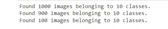
# Creating batches of the train, valid and test images and Pre-processing using mobilenet preprocess model

train_batches = ImageDataGenerator(preprocessing_function=tf.keras.applications.mobilenet.preprocess_input).flow_from_directory(

directory=train_path, target_size=(224,224), batch_size=10, shuffle=True)

valid_batches = ImageDataGenerator(preprocessing_function=tf.keras.applications.mobilenet.preprocess_input).flow_from_directory(

directory=valid_path, target_size=(224,224), batch_size=10, shuffle=True)

test_batches = ImageDataGenerator(preprocessing_function=tf.keras.applications.mobilenet.preprocess_input).flow_from_directory(

directory=test_path, target_size=(224,224), batch_size=10, shuffle=False)

We used the ImageDatagenerator that takes an argument preprocessing_function in which we applied preprocessing to the images which are provided by the MobileNet model.

Then using the flow_from_directory function, we provided the path of the directories and dimensions in which our image should be trained because the MobileNet model was trained for the images having dimensions 224x224.

Then defined the batch size and it can be defined as how many images can go in one iteration and then we shuffled the images. Image shuffling for test data was not applied because testing data will not be going for training.

After running the above cell in Jupyter Notebook or Google Colab, you will see the result like the following.

The general use case of the ImageDataGenerator is for augmenting the data and below is the guide for performing data augmentation using Keras ImageDataGenerator.

An Intuitive Guide On Data Augmentation In Deep Learning – Techniques With Examples

Creating model

Before fitting the training and validation data into the model, the deep learning model MobileNet needs to be fine-tuned by adding the output layer, removing the unnecessary layers, and making some layers non-trainable for better accuracy.

The following code will download the MobileNet model from Keras and store it in the mobile variable. You need to connect to the internet the first time running the following cell.

1	mobile = tf.keras.applications.mobilenet.MobileNet()

If you run the following code, then you’ll see the summary of the model in which you can see the series of layers of neural networks.

1	mobile.summary()

Now, we’ll add the dense output layer with a unit of 10 into the model because there will be 10 outputs from 0 to 9. Additionally, we removed the last six layers from the MobileNet model.

# Removing last 6 layers and adding our output layer

x = mobile.layers[-6].output

output = Dense(units=10, activation='softmax')(x)

Then we added all the input and output layers into the model.

1	model = Model(inputs=mobile.input, outputs=output)

Now, we are making the last 23 layers to be non-trainable and it’s an arbitrary number. This specific number has been achieved through many trials and errors. The sole purpose of this code is to better the accuracy by making some layers non-trainable.

# We are not going to train last 23 layers and it's an arbitrary number

for layer in mobile.layers[:-23]:

layer.trainable=False

If you see the summary of the fine-tuned model, then you’ll notice some differences in the number of non-trainable params and layers as compared to the original summary that you’ve seen earlier.

1	model.summary()

Now we are compiling the optimizer named Adam with learning rate 0.0001 along with loss function and metrics to measure the accuracy of the model.

1	model.compile(optimizer=Adam(learning_rate=0.0001), loss='categorical_crossentropy', metrics=['accuracy'])

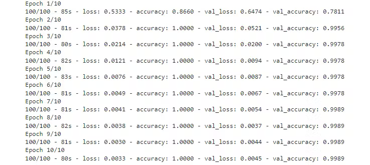
It’s time when the model is ready to train on the training and validation data. In the following code, we fed the training and validation data along with the number of epochs. The verbose is nothing but to display the accuracy progress and you can specify the numbers 0, 1, and 2.

1 2	# Running 10 epochs model.fit(x=train_batches, validation_data=valid_batches, epochs=10, verbose=2)

If you will run the above cell, then you’ll see every step of the epoch with training data’s loss and accuracy. You’ll see the same for validation data.

Steps of the epochs showing accuracy and validation accuracy

Saving the model

The model is now ready with an accuracy score of 99 percentile. Now keep one thing in mind this model is probably overfitted and might not perform well for images other than images of the dataset.

# Checking if the model exist otherwise save the model

if os.path.isfile("D:/SACHIN/Models/Hand-Sign-Digit-Language/digit_model.h5") is False:

model.save("D:/SACHIN/Models/Hand-Sign-Digit-Language/digit_model.h5")

The above code will check if there is already a copy of the model and if not then the save function will save the model in the specified path.

Testing the model

The model is trained and ready for recognizing images. This segment will cover loading the model and making functions for image preparation, predicting results, and displaying and printing the predicted result.

Before writing any code, some libraries that will be used further in the code need to be imported.

import numpy as np

import matplotlib.pyplot as plt

from PIL import Image

Loading the custom model

The prediction on images will be made using the model that was created above using the transfer learning technique, so first, it needs to be loaded for usage.

1	my_model = load_model("D:/SACHIN/Models/Hand-Sign-Digit-Language/digit_model.h5")

Using the load_model function, the model has been loaded from the specified path and stored inside the my_model variable for further use ahead in the code.

Preparing input image

Before giving any image for predicting or recognizing to the model, it needs to be in the format that the model wants it.

def preprocess_img(img_path):

open_img = image.load_img(img_path, target_size=(224, 224))

img_arr = image.img_to_array(open_img)/255.0

img_reshape = img_arr.reshape(1, 224,224,3)

return img_reshape

First, we defined a function preprocess_img that takes the path of the image and then we loaded that image using the load_img function from the image utility and set the target size of 224x224, then converted that image into an array and divided that array by 255.0 which converted the pixels of the image between 0 and 1 and then reshaped that image array into the shape (224, 224, 3) and finally returned that reshaped image.

Predicting function

def predict_result(predict):

pred = my_model.predict(predict)

return np.argmax(pred[0], axis=-1)

Here, we defined a function predict_result that takes predict argument which is basically a preprocessed image and then used the predict function to predict the result and then returned the maximum value from the predicted result.

Understanding numpy.argmax() Function In Python

Display and predict image

First, there’ll be a function that will take a path of the image and then display the image and the predicted result.

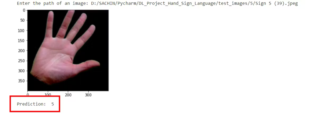
# Function to display and predicting the Image

def display_and_predict(img_path_input):

display_img = Image.open(img_path_input)

plt.imshow(display_img)

plt.show()

img = preprocess_img(img_path_input)

pred = predict_result(img)

print("Prediction: ", pred)

The above function display_and_predict takes the path of an image and used the Image.open function from the PIL library to open the image and then used the matplotlib library to display the image, and then for printing the predicted result the image is passed to the preprocess_img function and then used the predict_result function to obtain the result and finally printed it.